Transformer

Recently, Open AI introduced its third version of language prediction model: GPT-3. The astonishing performance of this autocomplete tool brought excitement and shock to the AI industry. The quality of the model built with 175 billion parameters is very impressive in a sense that it produces human-like outputs. With GPT-3, people built a question-based search engine, HTML generation based on text descriptions, medical question answering machine, and even image autocompletion.

Two year ago, a new embedding technique shocked the world. BERT (Bidirectional Encoder Representations from Transformers) achieved state-of-the-art performance on numerous NLP tasks.

The two NLP models have one thing in common. (Hint: GPT, BERT) They are built upon transformer network.

Transformer

To understand how transformer works,

Multiprocessing with Python

Handling Big Data

Working with big data is a stressful job, especially when it involves a massive amount of computation. For example, training neural networks or dealing with gigabytes of data would be time-consuming. When it comes to enhancing the performance speed of high complexity tasks, there are two approaches: Vertical Scaling and Horizontal Scaling.

Vertical Scaling is an approach that refers to adding more power to the existing computing power. Buying better hardware using it can ensure faster computing. Instead of delivering many packages with a single bike, using a truck would be more efficient.

Horizontal Scaling uses more computing instances to tackle this problem. By dividing the work and assigning it to multiple computers, the task can be finished faster. Think of it as dividing packages and delivering them with multiple bicycles.

In this post, we will talk about parallel processing which is a horizontal scaling approach to solve tasks with high time complexity.

Multiprocessing

Python has a bult-in function called multiprocessing . The module enables users to perform their tasks in a parallel manner by taking advantage of multi-core CPUs.

Let’s take a look at the code below:

Sequential Processing

import time

# starting time
start = time.time()

# save the factorial results here
s_results = []

# add all integers from 1 to 1_000_000
def factorial(i):
    x = 1
    for k in range(1,i+1):
        x = x*k
    results.append(x)

# number of test cases
cases = [x for x in range(0,2001)]
for c in cases:
    factorial(c)

print("%s seconds" % (time.time()-start))

> 0.5778999328613281 seconds

Parallel Processing (using multiprocessing library)

import multiprocessing as mp
import time

# starting time
start = time.time()

# save the factorial results here
p_results = []

# calculate factorial of a number
def factorial(i):
    x = 1
    for k in range(1,i+1):
        x = x*k
    p_results.append(x)

# factorials from 1 to 2000
cases = [x for x in range(1,2001)]

######################
### The Difference ###
pool = mp.Pool(processes=5) # Number of processes that you want to use
pool.map(factorial, cases)
pool.close()
pool.join()
######################

print("%s seconds" % (time.time()-start))

> 0.222374095917 seconds

Confirming the results are equal

s_results == p_results

> True

However, parallel processing is not always faster than serial processing. The performance depends on the number of iterations. Parallel programming is efficient when each iteration is sufficiently expensive compared to processor time

Comparing sequential and parallel running time of factorial() (Optional)

Let’s prove whether parallel programming is not always faster than sequential programming:

Create running time data for comparison (This takes a while; took me about 20 minutes to run)

import multiprocessing as mp
import time

# calculate factorial of a number
def factorial(i):
    x = 1
    for k in range(1,i+1):
        x = x*k

# measuring computation time for seq and parallel
seq_times = []
prl_times = []

for i in range(101,2501):
    cases = [x for x in range(1,i)]
  
  # Sequential
  # starting time
    seq_start = time.time()
    for c in cases:
        factorial(c)
    seq_times.append(time.time()-seq_start)
        
  # Parallel
    prl_start = time.time()
    pool = mp.Pool(processes=5) # Number of processes that you want to use
    pool.map(factorial, cases)
    pool.close()
    pool.join()
    prl_times.append(time.time()-prl_start)

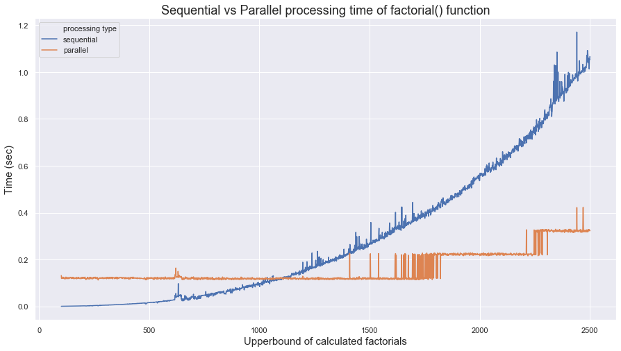
import seaborn as sns
import pandas as pd

fac = [i for i in range(101,2501)]

df = pd.DataFrame(data={"upper limit":fac,
                        "sequential":seq_times,
                        "parallel":prl_times})

df = df.melt(id_vars="upper limit",value_name="time",var_name="processing type")

sns.set(rc={'figure.figsize':(15,8)})
ax = sns.lineplot(x=df["upper limit"], y=df["time"], hue=df["processing type"])
ax.axes.set_title("Sequential vs Parallel processing time of factorial() function",fontsize=18)
ax.set_xlabel("Upperbound of calculated factorials",fontsize=15)
ax.set_ylabel("Time (sec)",fontsize=15)

As shown in the output image above, parallel processing is faster than sequential processing when the number factorials required to compute exceeds approximately 1100. The takeaway here is that parallel processing is only useful when the computation load is sufficiently expensive compared to the processor time.

Regularization

Supervised Learning can be explained as a process of finding the optimal weights of input features (predictors) to get the pre-determined outcome (labels). We tune hyperparameters, preprocess data and incorporate statistical methods to calculate weight of each variables that you feed to the model.

Meanwhile, one of the most important concerns when training a Machine Learning model is overfitting. This happens when your model is too complex that it performs extremely well on the train set, but poorly on the test set.

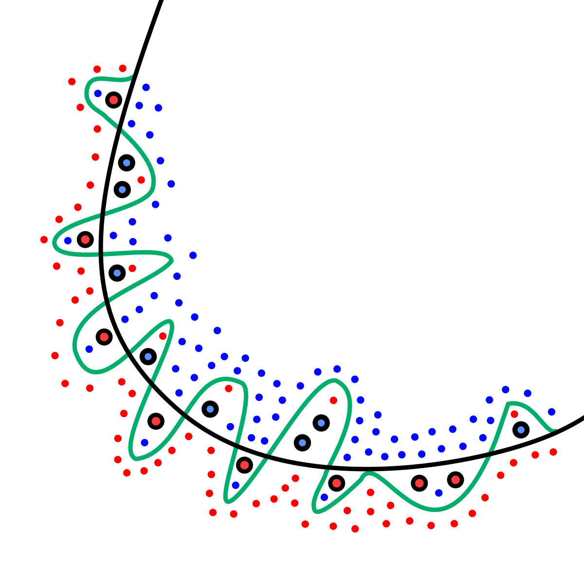
The image below illustrates an intuitive difference between a complex model (blue line) and a simple model (green line).

There are various methods that have been studied to prevent overfitting, which includes hyperparameter tuning, cross-validation, selecting features, and ensembling. Among the techniques, a way to fight overfitting by directly referring to the weights is called regularization.

Regularization

Overfitting is relevant to the number of weights or the size of weights. The number of weights implies the number of variables we are using for feeding the model. As we use more variables in the model, the dimension of weight space will increase as well as the complexity of the model. Small size of weights are also desirable to prevent overfitting, because large weights can cause rapid change in the model just like the green curve.

The bottom-line of how regularization works is that it punishes the loss function by taking number or size of weights into account. Of course, the method varies by how it penalizes the loss function

$L_0, L_1, L_2$ Regularization

The name of $L_0, L_1, L_2$ regularization is derived from the types norm applied to the weight vector. The penalization is done by adding these terms to the loss function.

In general, we define model as :

\(\hat{y} = \textbf{w}^T\textbf{x}\),

• $\textbf{w} = (w_1,w_2,w_3,…w_n)$ : weight vector
• $\textbf{x} = (x_1,x_2,x_3,…x_n)$ : vector of selected features or variables.
• $f$: loss function

The loss would be $f(y - \hat{y}) = f(y-\textbf{w}^T\textbf{x})$ and minimizing this would be the objective of machine learning. The regularization modifies this loss by adding the norm:

($\lambda$ is the degree of penalization or strength of regularization. This is also a hyperparameter.)

$L_0$ norm​ ($\vert\vert\textbf{w}\vert\vert_0$) is the number of non-zero elements in a vector:

$L_0 \ regularization = f(y - \textbf{w}^T\textbf{x}) + \lambda \vert\vert \textbf{w}\vert\vert_0$

$L_1$ norm ($\vert\vert\textbf{w}\vert\vert_1$) is the sum of absolute values in a vector:

$L_1 \ regularization = f(y - \textbf{w}^T\textbf{x}) + \lambda\vert\vert\textbf{w}\vert\vert_1$

$L_2$ norm ($\vert\vert\textbf{w}\vert\vert_2$) is the squared root of the sum of squared values in a vector. $L_2$ regularization uses squared value of $L_2$ norm:

$L_2 \ regularization = f(y - \textbf{w}^T\textbf{x}) + \lambda\vert\vert\textbf{w}\vert\vert^2_2$

Intuitions & Comparison between Regularization Methods

• Using $L_1$ regularization in linear regression is called Lasso regression, while using $L_2$ regularization is called Ridge regression
• $L_0$ method promotes using less amount of features, so it can be used as a feature selection method.
• $L_1$ method encourages non-necessary feature weights to be zero. As you strengthen the regularization power (increasing $\lambda$), features with small weights will be zero. Thus, we can use $L_1$ regularization as feature selection, just like $L_0$. Also, $L_1$ is more robust than $L_2$ because it is less sensitive to outliers. However, $L_1$ does not have a unique solution.
• $L_2$ method is less sensitive to data compared to $L_1$. Sensitive here means that the weights remain fairly consistent when there is a small adjustment to the data points. Also, because it is a convex the solution is unique when minimizing it. Thus it is computationally efficient. Unlike $L_0, L_1$, because $L_2$ does not completely make weights to 0, it can be a bit sensitive to irrelevant variable or features.
• In regularization scale and units of variables matter a lot.
• The overfitting occurs, because we do not have all data. Thus, the effect of regularization will go down as the training data size increases.

Elastic Net

Elastic net is a regularization method with $L_1$ and $L_2$ combined:

$f(y - \textbf{w}^T\textbf{x}) + \lambda(\alpha\vert\vert\textbf{w}\vert\vert_0+ (1-\alpha)\vert\vert\textbf{w}\vert\vert^2_2)$

• $\lambda$ control the strength of regularization

• $\alpha$ controls the relative strength of each regularization method
• L1 promotes sparsity (less weight number) and the L2 promotes smoothness.
• The functional is strictly convex, so the solution is unique.

Information Extraction Methodologies

In the previous post, I explained the process and importance of Information Extraction (IE). In this post, detailed methodologies and approaches to IE will be covered.

The methodologies can be classified into three learning based approaches:

1. Rule Learning based

2. Classification based

3. Sequential Labeling based

Traditionally, all of these approaches are considered as a supervised learning because labeled data is required to train the model for extracting information.

Rule Learning based Method

This approach is self-explanatory: we define a set of rules or patterns to extract information. In general, the rule learning based methods have three ways of learning:

• Dictionary-based (Pattern-based)
• Rule-based
• Wrapper induction

Dictionary-based (Pattern-based) approach creates a predefined template (dictionary) and use it to extract required information from the new texts. The core issue to this approach is how to detect patterns and construct the dictionary. Extraction takes place when the dictionary finds a triggering word (usually a verb) and tries to locate the target entities by identifying its pattern.

For example, let’s say we want to extract information of primary habitats of different animals. We can include pattern “noun-verb-target” in our dictionary to extract information from the following sentence: “Bats live in a cave”. In this case, the triggering word would be “live”. Because “live” was in the sentence, the model would search for noun and target in the sentence and retrieve “cave” as the primary habitat for “Bats”.

Rule-based approach use several general rules rather than dictionary. The rules are related to syntaxes and semantics of the words delimiting the targeted entity. Usually two types are rules are included in the model: tagging rules and additional rules for correction or improvement. Tagging rules may include part-of-speech tagging, name entity and type of the word. Using this information, a specific word can be acknowledged as a target for extraction if it matches all the pattern.

For example, let’s reuse the example from the Dictionary based approach. In this case, we will create a table of rules as below:

Using the rules above, we can extract information by parsing following sentence: “Dragons live in a cave”. Because the word “cave” is a noun, word and place, it matches our rule in the table above. Thus, we can extract the habitat “cave”. However, we need to update our rules or generalize the rules to extract “Dragons” because the word is not in the rule table.

Wrapper induction is for semi-structured documents like html texts. Using the tag names or html, specific information can be retrieved from a constructed web page. For example, let’s say we have a html code as below:

<tbody>
  <tr></tr>
    <td class="title">Star Wars</td>
    <td class="ratings">5.3</td>
  <tr></tr>
    <td class="title">Jumanji 2</td>
    <td class="ratings">6.6</td>
  <tr></tr>
    <td class="title">Frozen 2</td>
    <td class="ratings">8.7</td>
  <tr></tr>
    <td class="title">Knives Out</td>
    <td class="ratings">9.1</td>
</tbody>

It is not hard to see that title of the movies are wrapped between <td class="title"> and </td>, while the ratings are in bewteen <td class="ratings"> and </td>. Using the wrappers and its characteristics (<td> and class namein this case) we can extract information from the html above.

The Rule Learning based Methods are intuitive, easy to understand and implement. However, require tedious manual labors of tagging and labeling the data. Largely pertaining to this characteristics, it is regarded as “a dead-end technology in academia while largely adopted by commercial vendors”.²

Classification based Method

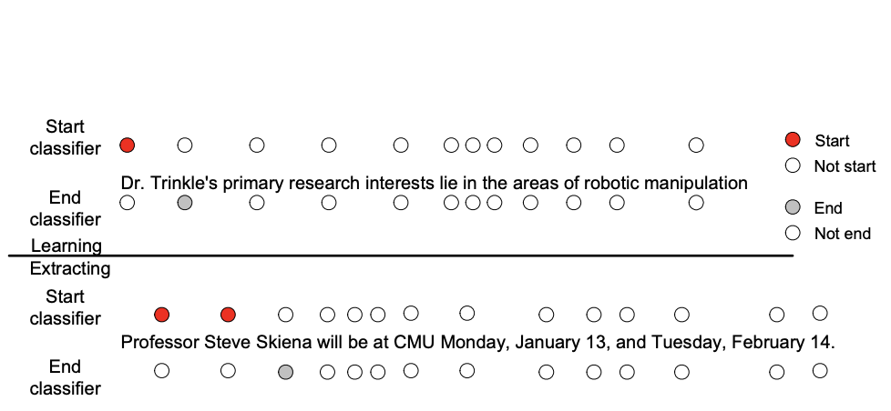
IE can be viewed as a classification problem; setting a boundary with two classifiers (starting classifier, end classifier) to locate an entity. Let’s look at the example below:

The words in the sentences are parsed as tokens and each words are classified by the starting classifier and ending classifier. Then, the result can be combined and entities of interest can be extracted.

There numerous machine learning classifiers available: Support Vector Machines, Random Forest Classifiers, Naive Bayes Classifier, etc. The classification based approach is about how to view or cast the IE problem as a classification problem. Choosing a classifier can follow after that.

Sequential Labeling based Method

Simlar to the Classification based method, we can view IE task as a sequantial labeling. Text data can be seen as a sequence of labeled tokens. Unlike other two methods, sequential labeling method allows the model to include context of dependencies between the words of interest. The sequential labeling method differs on how the conditional probability is computed since the objective is to find a label sequence $y$ that maximizes the conditional probability, $p(x \vert y)$.

Among the various methods, Conditional Random Fields are an important and widely incorporated model in the field of IE.

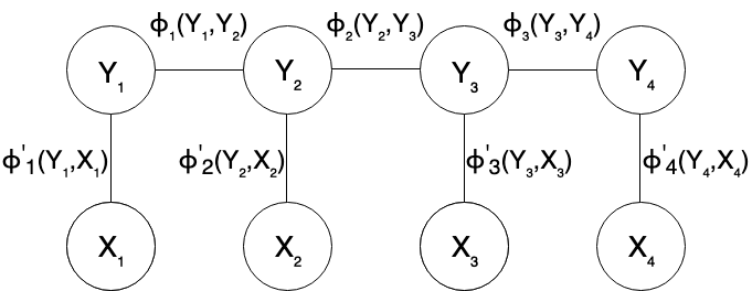
Conditional Random Field (CRF)

CRF is a type of discriminative undirected probabilistic graphical model. The important feature that CRF has is that it can include the information of “context” into the model, using dependencies between the tokens.

The definition follows:

Let $G = (V,E)$ be a graph such that $\mathbf{Y} = (Y_v)_{v \in V}$ so that $\mathbf{Y}$ is indexed by the vertices of $G$. Then $(\mathbf{X},\mathbf{Y})$ is a conditional random field when the random variables $Y_v$, conditioned on $\mathbf{X}$ obey the Markov property with respect to the graph:

$p(\mathbf{Y}_v \vert \mathbf{X},\mathbf{Y}_w, w\neq v) = p(\mathbf{Y}_v \vert \mathbf{X},\mathbf{Y}_w, w \sim v)$ where $w \sim v$ means that $w$ and $v$ are neighbors in $G$ ³

References & Citations:

^{1 Tang, Jie, et al. “Information extraction: Methodologies and applications.” Emerging Technologies of Text Mining: Techniques and Applications. IGI Global, 2008. 1-33.}

^{2 Chiticariu et al., “Rule-Based Information Extraction is Dead! Long Live Rule-Based Information Extraction Systems!”, Proceedings of the 2013 Conference on Empirical Methods in Natural Language Processing, 2013. 827–832}

^{3 Lafferty, J., McCallum, A., Pereira, F. (2001). “Conditional random fields: Probabilistic models for segmenting and labeling sequence data”. Proc. 18th International Conf. on Machine Learning. Morgan Kaufmann. pp. 282–289.}

Information Extraction

What comes to your mind when you think about data? Numbers? Fancy graphs? Nicely organized Excel tables and spreadsheets? The first thing that appears in my head is a messy table with lots of missing values and unstructured texts. The big data that media and people are talking about mostly refers to unstructured data; Approximately, 75-85% of data is unstructured, primarily text.¹ Although the figures may have variations, the takeaway here is that most of what we call “the big data” is a raw material; we have to mine and extract it to make it useful.

Unstructured Data

We see unstructured data everyday. Our emails, text messages, comments, audio files, video, etc. Although there are useful information in those data, it is difficult to process or gain insights from them. This is because they are ambiguous and have different contexts. Unlike structured data which has metadata like pre-defined fields (columns), unstructured data doesn’t have a fixed format or “description data of the data”. This makes the data searchable for machines and put them into algorithms or models.

Let’s look at the example below:

The unstructured data is just a plain text. We can read it and process the information in our head. There are 4 people described in this text and this contains information about their age, id and pursuing degree. However, we cannot search through this data using our computers. Computer needs index and column to retrieve search results. If we want to search for Robert’s age, we just have to run SQL queries to fetch his name like this SELECT Age FROM TABLE_NAME WHERE Name="Robert;"

This is what makes unstructured data and structured data different. In short, we have to extract information from the unstructured data and convert it to structured data.

This is the field in Natural Language Process, Information extraction.

Information Extraction

Information Extraction (IE) refers to the process of automatically retrieving structured information from unstructured data. It can be regarded as a pre-requisite step for analyzing unstructured data. This term is distinct from Information Retrieval (IR), which is more relevant to the “querying” or “searching” documents based on some set of keywords.

General Architecture, Process, Subtasks of Information Extraction

Information Extraction includes following subtasks according to its nature of problem:  

• Named Entity Recognition (NER)

  Recognizing known entity names such as people, places, numerical expression. The task focuses on identifying the entity and extracting it. For example, “Jake lives in Canada” can be processed into extracting “Jake” as a person and “Canada” as a location.

• Named Entity Linking (NEL);Named Entity Disambiguation (NED)

  Named Entity Linking is getting entities from NER and matching it to the knowledge that you already have in the database. It is a task of finding what the entity actually means in terms of the context. For example, from the sentence “Tom is one of the best actors in history. He showed excellent performance on Mission Impossible series”, NER system will recognize Tom as a person. However, it doesn’t know whether this is Tom Cruise or Tom Hanks. Named Entity Linking will retrieve knowledge from the existing database to find answer to this problem using the context.

   

• Temporal Information Extraction (Event Extraction)

  The purpose of Temporal Information Extraction is to identify events. Detecting certain frequency, dates, recognizing who is involved and what is happening. For example from the sentence, “Yesterday Jake hurt his leg so he won’t play soccer tomorrow “, Yesterday and tomorrow is the temporal information and we can structure our data by putting these information into date and matching description according to the date: Yesterday : hurt his leg , tomorrow : won’t play soccer.

• Relation Extraction (RE)

  This task is pretty much self-explanatory; it is about figuring out relationship between entities. For example, from the sentence, “Jake studies in UBC” information such as PERSON studies in LOCATION can be extracted.

• Coreference Resolution (CR)

  This is a task specifically for detecting entities called in different names. For example, “Microsoft” and “MS” refers to the same entity but in different ways. CR tries to find all expression that respective entities have.

Methodologies/Approaches

Also, there are several types of approaches and methodologies to Information Extraction²:

• Rule Learning based Extraction Method
• Classification based Extraction Method
• Sequential Labeling based Extraction Method
• Non-linear CRF (Conditional Random Fields) based Extraction Method

(I will discuss each approaches on individual posts)

References & Citations:

^{1 http://breakthroughanalysis.com/2008/08/01/unstructured-data-and-the-80-percent-rule/}

^{2 Tang, Jie, et al. “Information extraction: Methodologies and applications.” Emerging Technologies of Text Mining: Techniques and Applications. IGI Global, 2008. 1-33.}