Bias-Variance Tradeoff

19 Sep 2019

Choose one? Low Bias vs. Low Variance

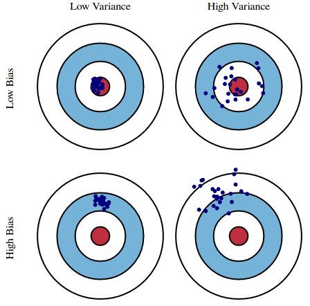
An archer tries to shoot 100 arrows to his target. Possible outcomes can be categorized like the image below:

source: https://pbs.twimg.com/media/CpWDWuSW8AQUuCk.jpg

 

Low bias refers to a situation where an archer’s shots are relatively close to the center of the target. Low variance refers to a situation where the archer’s shots were well-clustered and consistent. A good archer would make his shots look like low bias and low variance; well-clustered shot at the center. This is exactly what our machine learning model should be trained to do.

The image above provides an intuitive definition of bias and variance. Bias in statistics is a difference between an expected value of the estimator and the “real” value of the estimated parameter. On the other hand, Variance refers to the fluctuations or spread of the model.

Bias occurs when you fail to learn from the training data. If the archer does not practice much, it is more probable that he would miss the center of the target. A high bias situation like this is called underfitting; your model fails to learn from the training data.

If the archer practices on his consistency of shooting, he would generate “low variance” result. The archer trains, the lesser spread of arrow shots would become. Suppose the archer trains only on a specific size and shape of the target. In this case, if the target changes archer would not be familiar with the target and generate low bias high variance result. This is because the archer trained too much on a specific shaped target and lost flexibility or adaptiveness. This is called overfitting; your model trains too much on the dataset, that it fails to predict or to show good performance in real tests.

Every machine learning model would aim for low bias and low variance. We want all of our arrows (estimation) to hit the very center of the target (real values). However, this is practically impossible, as variance and bias are in a “tug of war” relationship. This is what we call trade-off.

Trade-off?

(feat. $3\choose2$ Your College Life)

Choose 2	Consequences
source	source

 

At some point of life, you might have seen this popular meme. Although it assumes that the three options have binary values (either you can have it or not) in a mutually exclusive way, it teaches the lesson that you can’t always have everything. In economics, this problem can be associated to opportunity cost, where “the loss of potential gain from other alternatives occurs when one alternative is chosen”$^1$ (In short, it’s a trade-off). Bias and Variance also have this type of “trade-off” relationship, in a supervised machine learning model.

(If you want to see a mathematical proof of how this works, check the bottom of this post)

Because low bias and variance for a model cannot be achieved at the same time, we have to make a compromise between variance and bias like the image below:

 

source: https://blog.naver.com/samsjang/220968297927?proxyReferer=https%3A%2F%2Fwww.google.com%2F

 

A Good Compromise

 

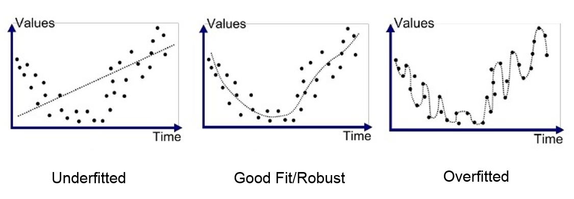
If we cannot achieve the low bias and variance at the same time, what should we do? Also, if this is the case we should consider the chance of overfitting (high variance low bias) and underfitting (high bias low variance), because the extreme minimization on one metric will maximize the other.

Generally, when your machine learning model is underfitted it will be simple. On the other hand, if you model is overfitted it will be very sophisticated. The visualizations below would help you understand this:

source: https://medium.com/greyatom/what-is-underfitting-and-overfitting-in-machine-learning-and-how-to-deal-with-it-6803a989c76

Unlike the college life trade-off meme, you have a choice to balance the two metrics. If bias and variance are well adjusted (in other words well compromised) the model would learn from the training data and be flexible enough to adapt to real data.

There aren’t any golden rules for deciding this, because there are many variables that affect this balance: characteristic of dataset, implemented algorithm, context of model application.

Here’s a simple lesson for you: ‘To go beyond is as wrong as to fall short’

Appendix

Proof using Mathematical Expression

Let’s assume that we try to fit a model $y = f(x) + \epsilon$. $y$ is our target variable and $f(x)$ is a true or real function that we want to approximate. $\hat{f}(x)$ is our model and $\epsilon$ is the noise with zero mean and variance $\sigma^2$. We want our model to be as accurate or close as the true function and “close” in mathematics are usually defined with a small difference. To achieve this, mean squared error between $y$ and $\hat{f}(x)$ is computed for minimization.

 

Objective: minimize $E[(y- \hat{f}(x))^2]$

• Bias of our function is: $ Bias[\hat{f}(x)] = E[\hat{f}(x)] - E[f(x)]$
• Variance of our functions is: $ Variance[\hat{f}(x)] = E[\hat{f}(x)^2] - E[f(x)]^2$

 

Let’s write

• $\hat{f}(x)$ as $\hat{f}$
• $f(x)$ as $f$

 

Because $y=f$, we can derive this equation like this:

 

Therefore:

$E[(y- \hat{f}^2]= (Bias[\hat{f}])^2 + Variance[\hat{f}] + \sigma^2$

• $\sigma^2$: irreducible error

Now, here’s the thing. We know that squared values are always non-negative, and variance is also non-negative. In this sense, the values in the equation are always non-negative. Since the left side of equation can be minimized and $\sigma^2$ is treated as a constant, only Bias and Variance are left to toggle. Therefore we know that if we reduce bias, variance increases and vice versa; it is a tug of war between the two variables.

TL;DR:

- Increasing bias will decrease variance

- Increasing variance will decrease bias

Citations:

$^1$ https://www.lexico.com/en/definition/opportunity_cost

References:

• https://web.stanford.edu/class/stats202/content/lec2.pdf
• https://en.wikipedia.org/wiki/Bias%E2%80%93variance_tradeoff
• https://www.opentutorials.org/module/3653/22071