Parametric vs Non-parametric
28 Sep 2019

Statistics have two main branches: descriptive statistics and inferential statistics.
Descriptive Statistics tries to “describe” the data by summarizing it with the use various measurements. For example, let’s say that you are a teacher responsible for 40 students in your class. How would you answer the questions like this?
- How tall are your students?
Are you going to name all the students and their height? This would be the most exact answer, but take a lot of time. Instead, you can say, “my students are 140cm in average, and they are all similar except for a few who are shorter”. This definitely does not tell all about your student’s height, but provides a ballpark figure. In terms of statistics, this answer is given by combining central tendency (average) and the spread or variability (all similar except for a few).
The other branch is Inferential Statistics, where “inference” or “prediction” is made with given data. Unlike descriptive statistics that focuses only on explaining the given data in an efficient and effective way, inferential statistics tries to go beyond the given data. Just like the image below:

source: https://eliamdur.com/index.php/2018/09/08/the-blind-men-and-the-elephant/ illustration by Hans Moller
The blind men are trying to guess what this “thing” is by touching a part of an elephant. In statistics, the elephant is population, which is the actual or whole picture that we are trying to infer. The parts of elephant that blind men are touching are samples. Simply saying, inferential statistics is about guessing the elephant from what you touch; inferring population from samples.
Finally, we are all on the same page now! Let’s talk about this post’s main topic: parametric vs non-parametric.
Parametric Statistics
“Parameter (Statistical Parameter; Population Parameter) is a quantity entering into the probability distribution of a statistics or a random variable” 1
Can you tell the difference between parameter and variable? This can be a first step of understanding the difference between parametric and non-parametric statistics.
- “Variables are quantities which vary from individual to individual.”2
- “Parameters do not relate to actual measurements, but to quantities defining a theoretical model”.3
Parameters are values that refer to specific family of distribution. It can be used to define model or altered to see how model changes. In short, we should not treat values from data as parameters.
Let’s look at the mathematical expression below:
\[X \sim N(3,2^2)\]
We consider 3 and 2 as parameters, but not as variables. This is because 3 and 2 are mean and variance that can define a particular distribution in the family of normal distribution. They are “quantities defining a theoretical model”, which in this case is a Gaussian distribution.
So, parametric statistics has assumption in its base line; the sample data is derived from a particular population distribution with a fixed number of parameters. Therefore, linear regression, logistic regression and student t-test are examples of parametric statistics.
Non-Parametric Statistics
If parametric statistics has assumption, is non-parametric statistics assumption-free?
No. Non-parametric statistics do not have assumptions in terms of distribution. It is true that non-parametric statistics has a fewer assumptions than parametric statistics, but there still are other assumptions depending on methods. (Lists of non-parametric methods)
Non-parametric methods are usually used when the data is in an ordinal variable or rank. Order statistics is a branch of non-parametric statistics that is relevant to this. You are advised to use non-parametric methods when:
- Sample size is small to risk making assumptions
- Data is not symmetric
- Data has too many important outliers. (When the median represents the central tendency better than the mean)
It’s Up to You
Usually, parametric statistics are favored over non-parametric statistics. This is because parametric statistics are more powerful than non-parametric ones, if the assumptions are correct. Because non-parametric methods do not make assumptions with distribution and according parameters, it is safer but less powerful. Using which type of statistics would differ by data, situation and context.
Just like everything else, choosing between the two statistics depends on the context, as there is no absolute rule in our world.
Citations
1 Kotz, S.; et al., eds. (2006), “Parameter”, Encyclopedia of Statistical Sciences, Wiley.
2 BMJ 1999;318:1667 (https://www.bmj.com/content/318/7199/1667)
3 BMJ 1999;318:1667 (https://www.bmj.com/content/318/7199/1667)
The Curse of High Dimension
22 Sep 2019
 source: https://cheezburger.com/8249495040
It’s a common knowledge that, we live in the 3-Dimensional space.
We know that line represents 1-dimensional space, the square represents 2-dimensional space and a cube represents 3-dimensional space. However, not many people would be able to tell the definition of dimension. Dimension is an inevitable topic to data science, as more and more variables are included in the datasets. This post will start with definition of dimension and discuss about the curse of dimension in Data Science.
Dimension
The dictionary meaning of dimension in general is “a measurable extent of some kind, such as length, breadth, depth or height”1. In this context, we can think of dimension as a way of representing particular physical quantities. Probably the most intuitive and easy way of explaining it is the definition below:
Dimension is the least number of coordinates required to describe any point within it. 2
| 1-Dimension |
2-Dimension |
3-Dimension |
| (x) |
(x,y) |
(x,y,z) |
More mathematical way of expressing this concept is:
When linearly independent vectors span $S$, dimension is the number of linearly independent vectors in the basis for $S$.
Still confused? Let’s look at this data then:
| Index |
Height(cm) |
Weight(kg) |
Foot size(mm) |
Waist Size(cm) |
Gender (M:1, F:0, O:2) |
| 0 |
175 |
80 |
265 |
83 |
1 |
| 1 |
180 |
68 |
280 |
79 |
1 |
| … |
… |
… |
… |
… |
… |
| 999 |
162 |
48 |
235 |
66 |
0 |
This data seems like a body measurement of a thousand people. There are height, weight, foot size and waist size. Let’s say that we want to predict the gender variable with the other four variables. What do you think the dimension of this data is?
Of course, including our dependent variable (or predicting variable), the dimension of this data is 5. We can create a vector with index 1 into (180,68,280,79,1). We can notice that the least number of coordinates required to describe this data is the number of variables. In a very simple way to put this, dimension of data corresponds to the number of variables in our analysis.
Sparsity: The Curse
When you perform data analysis, there is a high chance that you will have more than 5 variables. In that case, your dimension would get larger. When dimensions get larger, the number of coordinates that it can cover grows exponentially. In other words, the matrix that you are working on would be a sparse matrix. (Most of the elements in the matrix are filled with 0). This means that amount of data need to generate good performance also grows exponentially. Moreover, the visualization would get much more harder when dimensions increase.
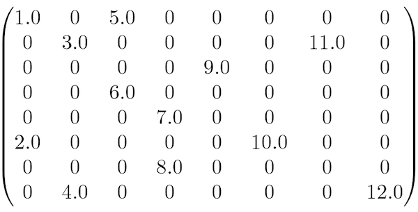 a sparse matrix
“A matrix is sparse if many of its coefficients are zero. The interest in sparsity arises because its exploitation can lead to enormous computational savings and because many large matrix problems that occur in practice are sparse”3
The curse that sparsity afflicts can be categorized into two perspectives: Space complexity and Time complexity
Space Complexity
If matrix is sparse, many of its elements are zero. This suggests that even though there are a little number of non-zero entries in the matrix, all the zeros should be stored into the computer memory as well. In short, memory would be definitely wasted by storing unmeaningful values, causing massive inefficiency in terms of storage. The larger the matrix and dimension gets, the more memory would be wasted in an exponential way.
Time Complexity
What if our machine learning model tries to perform operations on the sparse matrix? Since most of the entries are zero-values, lots of time will be spent on doing meaningless calculations with zeros. This can be problematic when our model is complex and requires many calculations.
Risk of Overfitting
High dimensionality also leads to the risk of overfitting the model. The more features we incorporate to the model, the more likely it is for the model to perform perfectly on the training data. This will make the model highly biased by even making it learn the noises in the data.
Citations:
1https://www.lexico.com/en/definition/dimension
2https://web.archive.org/web/20140111191053/http://curious.astro.cornell.edu/question.php?number=4
3pg.1, Direct Methods for Sparse Matrices, Second Edition, 2017.
References:
-
https://web.stanford.edu/class/stats202/content/lec2.pdf
-
https://en.wikipedia.org/wiki/Bias%E2%80%93variance_tradeoff
-
https://www.opentutorials.org/module/3653/22071
-
Direct Methods for Sparse Matrices](http://amzn.to/2DcsQVU), Second Edition, 2017
-
https://machinelearningmastery.com/sparse-matrices-for-machine-learning/
Bias-Variance Tradeoff
19 Sep 2019
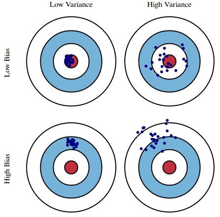
Choose one? Low Bias vs. Low Variance
An archer tries to shoot 100 arrows to his target. Possible outcomes can be categorized like the image below:
source: https://pbs.twimg.com/media/CpWDWuSW8AQUuCk.jpg
Low bias refers to a situation where an archer’s shots are relatively close to the center of the target. Low variance refers to a situation where the archer’s shots were well-clustered and consistent. A good archer would make his shots look like low bias and low variance; well-clustered shot at the center. This is exactly what our machine learning model should be trained to do.
The image above provides an intuitive definition of bias and variance. Bias in statistics is a difference between an expected value of the estimator and the “real” value of the estimated parameter. On the other hand, Variance refers to the fluctuations or spread of the model.
Bias occurs when you fail to learn from the training data. If the archer does not practice much, it is more probable that he would miss the center of the target. A high bias situation like this is called underfitting; your model fails to learn from the training data.
If the archer practices on his consistency of shooting, he would generate “low variance” result. The archer trains, the lesser spread of arrow shots would become. Suppose the archer trains only on a specific size and shape of the target. In this case, if the target changes archer would not be familiar with the target and generate low bias high variance result. This is because the archer trained too much on a specific shaped target and lost flexibility or adaptiveness. This is called overfitting; your model trains too much on the dataset, that it fails to predict or to show good performance in real tests.
Every machine learning model would aim for low bias and low variance. We want all of our arrows (estimation) to hit the very center of the target (real values). However, this is practically impossible, as variance and bias are in a “tug of war” relationship. This is what we call trade-off.
Trade-off?
(feat. $3\choose2$ Your College Life)
At some point of life, you might have seen this popular meme. Although it assumes that the three options have binary values (either you can have it or not) in a mutually exclusive way, it teaches the lesson that you can’t always have everything. In economics, this problem can be associated to opportunity cost, where “the loss of potential gain from other alternatives occurs when one alternative is chosen”$^1$ (In short, it’s a trade-off). Bias and Variance also have this type of “trade-off” relationship, in a supervised machine learning model.
(If you want to see a mathematical proof of how this works, check the bottom of this post)
Because low bias and variance for a model cannot be achieved at the same time, we have to make a compromise between variance and bias like the image below:

source: https://blog.naver.com/samsjang/220968297927?proxyReferer=https%3A%2F%2Fwww.google.com%2F
A Good Compromise
If we cannot achieve the low bias and variance at the same time, what should we do? Also, if this is the case we should consider the chance of overfitting (high variance low bias) and underfitting (high bias low variance), because the extreme minimization on one metric will maximize the other.
Generally, when your machine learning model is underfitted it will be simple. On the other hand, if you model is overfitted it will be very sophisticated. The visualizations below would help you understand this:
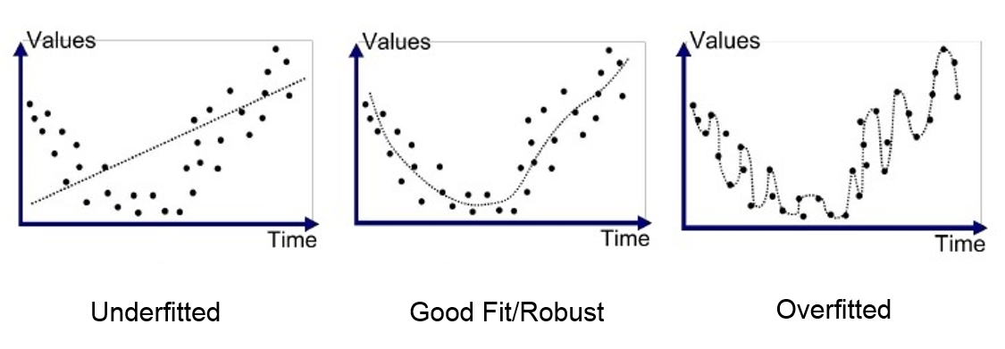
source: https://medium.com/greyatom/what-is-underfitting-and-overfitting-in-machine-learning-and-how-to-deal-with-it-6803a989c76
Unlike the college life trade-off meme, you have a choice to balance the two metrics. If bias and variance are well adjusted (in other words well compromised) the model would learn from the training data and be flexible enough to adapt to real data.
There aren’t any golden rules for deciding this, because there are many variables that affect this balance: characteristic of dataset, implemented algorithm, context of model application.
Here’s a simple lesson for you: ‘To go beyond is as wrong as to fall short’
Appendix
Proof using Mathematical Expression
Let’s assume that we try to fit a model $y = f(x) + \epsilon$. $y$ is our target variable and $f(x)$ is a true or real function that we want to approximate. $\hat{f}(x)$ is our model and $\epsilon$ is the noise with zero mean and variance $\sigma^2$. We want our model to be as accurate or close as the true function and “close” in mathematics are usually defined with a small difference. To achieve this, mean squared error between $y$ and $\hat{f}(x)$ is computed for minimization.
Objective: minimize $E[(y- \hat{f}(x))^2]$
- Bias of our function is:
$ Bias[\hat{f}(x)] = E[\hat{f}(x)] - E[f(x)]$
- Variance of our functions is:
$ Variance[\hat{f}(x)] = E[\hat{f}(x)^2] - E[f(x)]^2$
Let’s write
- $\hat{f}(x)$ as $\hat{f}$
- $f(x)$ as $f$
Because $y=f$, we can derive this equation like this:

Therefore:
$E[(y- \hat{f}^2]= (Bias[\hat{f}])^2 + Variance[\hat{f}] + \sigma^2$
- $\sigma^2$: irreducible error
Now, here’s the thing. We know that squared values are always non-negative, and variance is also non-negative. In this sense, the values in the equation are always non-negative. Since the left side of equation can be minimized and $\sigma^2$ is treated as a constant, only Bias and Variance are left to toggle. Therefore we know that if we reduce bias, variance increases and vice versa; it is a tug of war between the two variables.
TL;DR:
- Increasing bias will decrease variance
- Increasing variance will decrease bias
Citations:
$^1$ https://www.lexico.com/en/definition/opportunity_cost
References:
- https://web.stanford.edu/class/stats202/content/lec2.pdf
- https://en.wikipedia.org/wiki/Bias%E2%80%93variance_tradeoff
- https://www.opentutorials.org/module/3653/22071
A Simple Guide to Github
13 Sep 2019
Git ?
Let’s assume that you have to submit a report as a group for your science class. In this case, you would want to split the works. Different roles and responsibilities can be assigned to each person. Some might focus on doing research and gathering information, some can just write with the collected information and others might do the presentation.
However, let’s say the professor required everyone in the team to take part in writing the report. In this case, many problems can be expected:
-
“Who wrote this paragraph?”
-
“I accidently deleted our file… do you have any backup files?”
-
A: “Hey I am done with my part. I will just have to merge mine with yours”
B: “Actually, I updated my stuff. I will send you a new version of my work”
-
A: “Hey your writing has some typos. I corrected them”.
B: “But I revised my part yesterday, and the content also changed”
A: “Why did you change it?”
B: “Because some of my contents were contradicting your part”
When it comes to a collaborative work and especially when the size of group gets bigger, it is hard to keep track of who did the work, and what the newest version of each other’s work is. Also, how to update the work and resolve conflicting contents can be confusing.
Git is “a free and open source distributed version control system designed to handle everything from small to very large projects with speed and efficiency”. Easily saying this, it is a software used to manage and control versions of your project. Also, it is very useful to keep track of who made the changes and updates. It also provides search functionality which facilitates your work. In terms of development, git is by far the most popular platform to do your coding projects.
Github is a platform where gits are uploaded. (Hub of gits!) It is “a code hosting platform for collaboration that lets you and others work together on projects from anywhere”, according to the service’s own introduction. Github users can share, review, collaborate, fork (copying and experimenting) on other’s projects. It is more like a social networking platform for developers too.
Installation
Check here for installation (the official git website)
How it works
In order to use git, you need to understand how git works. Here are some new words that you should get used to:
- Local Repository
- Remote Repository
- Staging Area (Index)
And the diagram below explains the basic flows of git:
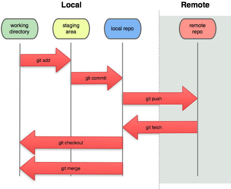 source: https://pismute.github.io/whygitisbetter
The local area is your computer that you are working on (probably where your git is installed). The remote area is the git server where your uploaded files are saved.
Repository is your project, a data structure that git has. If you want to start a new project, you have to create a new repository. Git controls the repository version by thinking of data like snapshots. It does not store the file itself, but remembers how it looked like.
Staging area is a simple file where the snapshots of your files are stored. It contains information about what changes to upload to the remote repository. Think of it as a purgatory before reaching heaven (Remote repository or Github server).
Creating Repository
There are two ways to create a repository:
- Create a repository on your local area (your computer) and initialize git. Then create a new repository on Github and use git commands to set the location of remote repository that you created on Github
- Create a repository on remote area (through Github.com) and git clone to local area
Step 2 seems simpler, but if you have an existing project that you would like to upload, first way would be more convenient.
Method 1. Uploading Existing Projects
First, you need a remote repository on Github to store your project. Sign in to Github, and go to repositories tab. (should be easy to find) Then, you will see this in your screen:
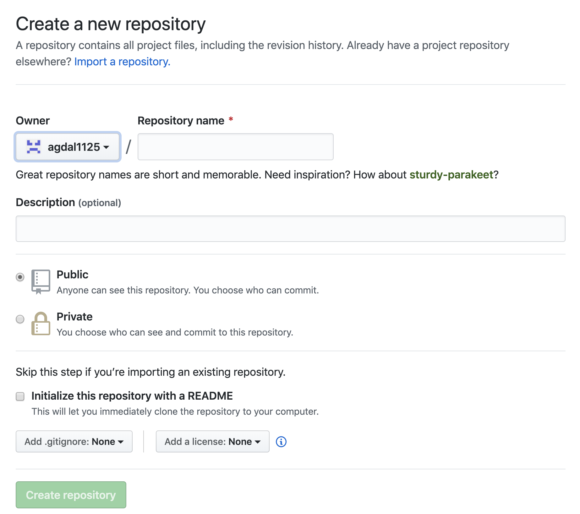
Fill in the repository name, description of your project and create the repository.
(**DO NOT CHECK **Initialize this repo with README)
Once you create your remote repository, you should be able to see a url that looks like this:

Remember this url because you need this to set your location of remote repository!
Finally, you are ready to upload your files from your local repository to remote repository. Just follow the command lines below:
# Change directory to the location of your project
$ cd /Desktop/your_project_directory/

# Initiate git
$ git init

# Add all the files in your current directory (staging)
$ git add .

# commit the files
$ git commit -m "Write any Comments or Notes"

# Locate your remote repository
$ git remote add origin git@github.com:username/project.git

# pushes the changes in local repo to remote repo
$ git push -u origin master
If you followed the steps successfully, you can go back to Github and check that your files are there!
Method 2. Creating a New Project
The process above is more complicated than this option. If you want to create a new project, you can create a remote repository and copy (clone/download) it into your local machine:
First, you need a remote repository on Github to store your project. Sign in to Github, and go to repositories tab. (should be easy to find) Then, you will see this in your screen:
Fill in the repository name, description of your project and create the repository.
(**CHECK **Initialize this repo with README)
Type in the commands below:
# Change directory to where your project should be
$ cd /Desktop/My_projects/Project_1/

# Clone remote repo into your local machine.
# This becomes your local repo
$ git clone git@github.com:username/project.git
Now, you will see that a folder was created with the same name of your remote repository on the Github. You can start your project there.
Updating Your Work
If you made changes to your project and want them updated to your remote repository, only three lines of codes are required:
# Add all the files in your current directory (staging)
$ git add .

# commit the files
$ git commit -m "Write any Comments or Notes"

# pushes the changes in local repo to remote repo
$ git push -u origin master
You can also make changes in the Github directly. However, if the changes are made in the remote repository directly, you would have to update your local repository. If you don’t, you won’t be able to commit or push your updates because the staging area sees that the “snapshots” they have in local repo is not consistent with the ones from remote repo. See the next section for how to resolve this problem.
Resolving Version Conflicts: Fetching/Pulling
If have a remote repository that has fresher version than your local repository. you will have to apply or make updates for the consistency of versions between the two repositories. In a short way, you need to download new stuffs on your local repository, just like a game patch. You cannot join and play others if you have an outdated version of your game. There are two ways of doing this:
$ git fetch origin

or

$ git pull origin master
Here’s a simple explanation. Pulling does more than fetching. It “fetches” and then “merges” to update your repository. Pulling “automatically merges the commits without letting you review them first”. If you are not involved in managing branches, pulling is recommended.
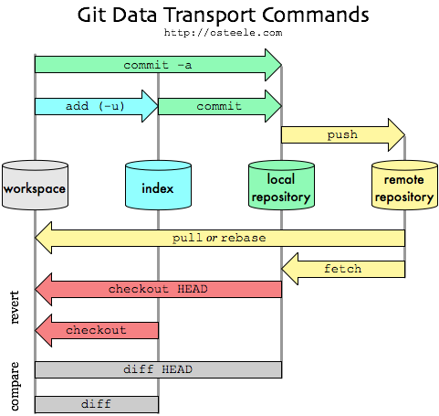
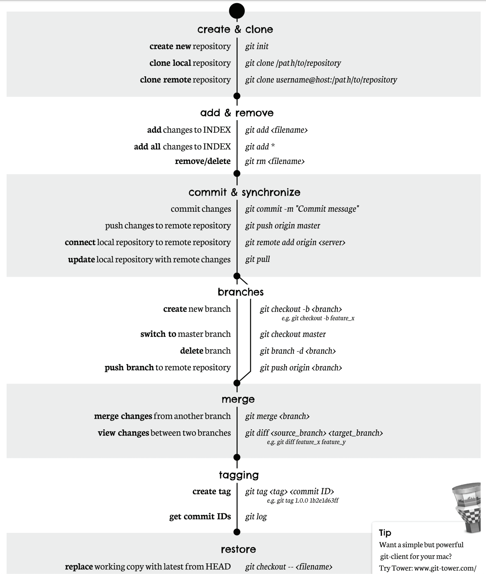
Github Cheatsheet
FYI, Here’s a cheatsheet of git command lines!
Resources & References:
- https://rogerdudler.github.io/git-guide/index.html
- https://kbroman.org/github_tutorial/pages/init.html
- https://help.github.com/en/articles/adding-an-existing-project-to-github-using-the-command-line
- https://stackoverflow.com/questions/292357/what-is-the-difference-between-git-pull-and-git-fetch
- https://blog.osteele.com/2008/05/my-git-workflow/
Data Manipulation with Pandas 2
04 Aug 2019
Pandas Tricks
In the previous post, basic usage of pandas was explained. In this post, more technical and useful tricks will be introduced. The following list of contents will be covered:
- Transpose
- Correlation
- Column Manipulation (re-ordering, re-naming, etc.)
There are many posts, books and even official documentations that explains how to make use of this wonderful library. In this post, I would like to discuss practical techniques and summarize the gist of pandas.
Transpose
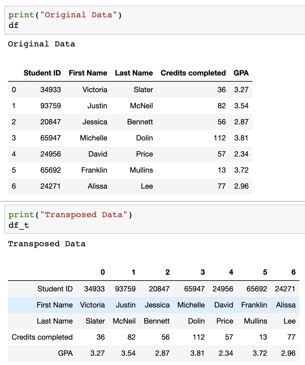
Let’s say you have data that looks like this:

Sometimes, you may want to switch rows and columns. This is when transpose function is used.
import pandas as pd

# Generate DataFrame
df = pd.DataFrame({"Student ID": [34933,93759,20847,65947,24956,65692,24271],
                  "First Name":["Victoria","Justin","Jessica","Michelle","David","Franklin","Alissa"],
                  "Last Name":["Slater","McNeil","Bennett","Dolin","Price","Mullins","Lee"],
                  "Credits completed":[36,82,56,112,57,13,77],
                  "GPA":[3.27,3.54,2.87,3.81,2.34,3.72,2.96]
                  })

# Transpose
df_t = df.transpose() # or  df.T  also works
You can see the result of the transpose as shown in the image below.
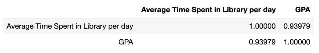
Calculating Correlation
In EDA(Exploratory Data Analysis), correlations between variables are essential statistical measures to gain insights from data. Pandas makes this calculation easy for us, with just a simple line of code.
import pandas as pd

# Generate example dataframe

df = pd.DataFrame({"Average Time Spent in Library per day":[1,2,3,4,5,6,7,8,9],
                  "GPA":[2.8,3.2,3.0,3.5,3.4,3.8,3.7,3.8,4.0]})

# Calculate correlation between the two columns

df.corr()
The .corr() function returns the result in a matrix form. The diagonal values of the matrix can be ignored as correlation of variable with itself is always 1. In this example, the correlation between the time you spend on library is highly correlated to your GPA or vice versa.
Remember that correlation does not guarantee any causal relationship. So use it wisely.
Column Manipulation, Operation
Just like Microsoft Excel, Pandas allows its users to generate new columns from existing columns (only If the columns have operatable data types)
import pandas as pd
# Generate example dataframes
df = pd.DataFrame({"Name":["A","B","C","D"],
"Income":[320000,240,380,23000],
"Currency":["KRW","EUR","CAD","JPY"]})
rate = pd.DataFrame({"Rate":[0.76,0.00084,0.0094,1.11],
"Currency":["CAD","KRW","JPY","EUR"]})
# Merge currency dataframe into df
df = df.merge(rate, how="left", on="Currency")
# Calculate income in USD using two columns Rate and Income
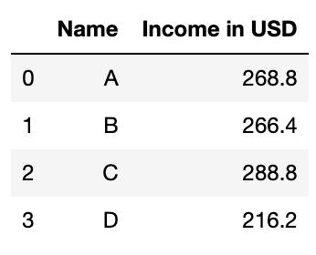
df["Income in USD"] = df["Income"]*df["Rate"]
# Let's see who earns the most
df[["Name","Income in USD"]]
So, we can see that person C earns the most.