Bayes' Probability

Bayes’ Theory

In probabilistic study, there are two main stream approaches:

1. Frequentist Approach( the classic probability )
   • Define probability as an event’s relative frequency in a large number of trials when performed infinite times
   • \[P(x) = \lim_{n_t -> \infty} \frac{n_x}{n_t}\]
   • \(n_t\) is total number of trials and \(n_x\) is number of that event \(x\) occurred and \(P(x)\) is the probability
   • However, application of frequentist approach is nearly impossible in the real word, because you cannot simply try everything infinite amount of times. It is difficult to apply real world problems…

1. Bayesian Approach
   • Define probability as a “degree of belief”. It is subjective, but not random
   • Experience and data are used to update the probability

   • Practical to apply in real world problems!!

   • Bayesian Theorem: \(P(H|E) = {P(H \bigcap E) \over P(E)} = \frac{P(E|H)*P(H)}{P(E)} = \frac{P(E|H)*P(H)}{P(H)*P(E|H) + P(H^c)*P(E|H^c)}\)

     • \(P(H)\) is called the prior probability, the probability that you know before the “update”

     • \(P(H \vert E)\) is called the posterior probability, the updated probability with new information

     • The Bayesian Theorem uses conditional probability to update prior probability to posterior probability

Conditional Probability

\(P(A \vert B) = {P(A \cap B) \over P(B)}\)

• Given that event B occurred, the chance that \(P(A)\) also occurred. (probability of A given B)
• if the two events A and B are completely independent, \(P(A \vert B) = P(A)\)
• This implies that information of B is irrelevant or useless when you want to know A

Example

Let’s say that a mother is in her 40s. She got a positive reaction from X-ray examination of breast cancer. What is her probability of really having a breast cancer?

• Probability that women in her 40s will have a breast cancer is 1%
• Probability that cancer patient of women in 40s will be diagnosed positive from X-ray examination is 90%
• Probability that healthy women in 40s will be diagnosed positive from X-ray examination is 5%

Solution

The probability that we want to know is \(P( c \vert p)\)

Given informations are:

• \(P(c)\) = 0.01
• \(P(p \vert c)\) = 0.9
• \(P (p \vert c^c)\) = 0.05

Using the Bayes theorem: \(P(c \vert p) = {P(c)*P(p \vert c) \over P(p)}\)

So all we need to know is the value of \(P(p)\) which is:

\(P(p) = P(p|c)*P(c) + P(p|c^c)*P(c^c) = 0.9*0.01 + 0.05*0.99 = 0.0585\)

The final calculation of what we want to know would be: 0.01 * 0.9 / 0.0585 = 0.15384…

Thus, the probability that a mother will have breast cancer, given that her X-ray examination was positive is about 15%

Topic Modeling and Latent Dirichlet Allocation

Topic Modeling

The objective of topic modeling is very self explanatory; discovering abstract “topics” that can most describe semantic meaning of documents. It is an integrated field of machine learning and natural language processing, and a frequently used text-mining tool to discover hidden semantic structures in the texts. Topic modeling can help facilitating organization of vast amount of documents and find insights from unstructured text data.

LDA (Latent Dirichlet Allocation)

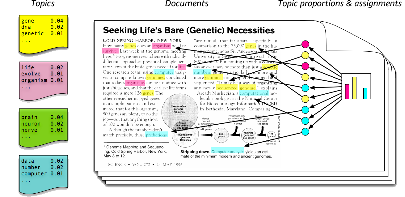
LDA is one of the graphical models used for topic modeling. LDA is a generative statistical model that posits specific probability of word appearance in accordance to a specific topic. The image below best explains how LDA works.

The key part of LDA lies in the right part of the diagram, “Topic proportions and Assignments”. LDA views documents as a mixture of various topics and each topic consists of a distribution of words. LDA has several assumptions:

• number of N words are decided by Poisson distribution
• from number K topic sets, document topics are decided by Dirichlet distribution
• each word \(w_{i}\) in the document is generated by following rules:
  1. pick a topic in accordance to the multinomial distribution sampled above
  2. generate the word using the topic in accordance to the multinomial distribution of the words in that topic

Model

• \(\alpha\) is the parameter of the Dirichlet prior on the per-document topic distributions,
• \(\beta\) is the parameter of the Dirichlet prior on the per-topic word distribution,
• \(\theta_{m}\) is the topic distribution for document \(m\),
• \(\varphi_{k}\) is the word distribution for topic \(k\),
• \(z_{mn}\) is the topic for the \(n\)-th word in document \(m\), and
• \(w_{mn}\) is the specific word.

TF-IDF

TF and IDF

Text Frequency (TF)

• TF is an index that shows frequency of words in each document in the corpus. It is simply calculated by the ratio of word counts by the total number of words in that document. Each word has its own TF value

Inverse Document Freqeucny (IDF)

• IDF is an index that shows the relative weight of words across all documents in the corpus. In other words, it is a representation of rarity of a word in the set of documents. Each word has its own IDF value

TF-IDF

• TF-IDF is a multiplication of TF and IDF values. It is a numerical statistics that aims to reflect significance of word in a particular document (TF), also considering other documents in the group (IDF).

Preprocessing

• Before you calculate the TF-IDF of all words, each documents need to be processed. They need to be tokenized
• Tokenizing is process of classifying sections of string and parsing them.
• For example, the text “He is a good boy” can be tokenized into: [“He”,”is”,”a”,”good”,”boy”]
• The processing methods can vary depending on stemming or lemmatization methods

Example code

# dependencies
import os
import nltk

work_dir = "/Users/nowgeun/Desktop/Research/Documents/"
text_files = os.listdir(work_dir)


def pre_processing(text):
    # lowercase
    text=text.lower()
    
    # remove tags
    text=re.sub("</?.*?>"," <> ",text)
    
    # remove special characters and digits
    text=re.sub("(\\d|\\W)+"," ",text)
    
    return text
    

def tokenize(text):
   tokens = nltk.word_tokenize(text)
    stems = []
    
    #pos(part of speech) tagging: grammatical tagging of word by their category (verb,noun,etc)
    for item in nltk.pos_tag(tokens):
        # Filtering tokens with only Nouns (N)
        if item[1].startswith("N"):
            if len(nltk.wordnet.WordNetLemmatizer().lemmatize(item[0])) == 1:
                pass
            else:
                stems.append(nltk.wordnet.WordNetLemmatizer().lemmatize(item[0]))

    return stems

# creating corpus from text files using preprocessing function 

token_dict = {}

for txt in text_files:
    if txt.endswith(".txt"):
        with open (work_dir+ txt) as f:
        
            data = "".join(f.readlines()).replace("\n"," ")
            data = pre_processing(data)

            token_dict[txt] = data    

TF-IDF computation using Scikit-Learn package

Example code

With Scikit-Learn package, you can compute the tf-idf value and retrieve the results as a matrix form.

• Each row of matrix represents respective documents
• Each column of matrix represents words that appear on all documents
• The matrix is sparse-matrix (where most values are 0). This is because not all words appear on all documents or the frequency of the word itself is very low

from sklearn.feature_extraction.text import TfidfVectorizer

vectorizer = TfidfVectorizer(tokenizer=tokenize, stop_words='english')

# matrix of all documents in rows and idf values of respective words in column
matrix = vectorizer.fit_transform(token_dict.values())

Web Crawling with BeautifulSoup

Webcrawling

Web crawling allows users to gather data directly from the internet. Web crawling is an act of software that explores world wide web (www) is an autonomous way to gather data. Portal’s search engines are based on these web crawlers that visits a myriad of web pages and collect data.

How it works

The internet is a collection of web pages formed by HTML (Hyper Text Markup Language). We navigate these HTML pages through browser (Chrome, Firefox, Safari, Internet Explorer, etc..) which facilitates exploration of web through Graphic User Interfaces (GUI) and various plugins. Web crawling is done by parsing the HTML, filtering necessary parts and saving them into files.

Cautions

• There may be legal penalties depending on the website that you wish to crawl
• Some websites has policies against web crawling (e.g. robots.txt contains information about data collection policy)
• Web crawling may cause traffic overload and this is pertinent to security issues

Basic Web Crawling with Python3

Required libaries: bs4, requests,

Simple Web Crawling

Simple web crawling can be achieved by using bs4 and requests libraries. The tricky part is in understanding structure of html and finding tags where the desired information belongs.

import requests
from bs4 import BeautifulSoup

# Connect to website via requests module
url = requests.get("your url that you wish to access")

# Retrieve html
html = url.text

# Parse the html data with BeautifulSoup
soup = BeautifulSoup(html, 'html.parser')

# You can see the HTML Raw Source code from the website that you have accessed
print(soup)


# Retrieving specific information, using html tags

### This retrieves the first html tag that has "div" tag and its class name "itemname"
print(soup.find("div",{"class":"itemname"))

### find_all function retrieves all tags that has "a" tag in the raw source codes
### shown as a list form
print(soup.find_all("a"))

### get_text() function retrieves only text information from the specified tags
soup.find("div",{"id":"item_number").get_text()

Student's T-test

Student’s T-Test

• Student’s t-test is one of statistical hypothesis tests which is performed when the test statistics is assumed to follow a Student’s t-distribution under the null hypothesis.
• It is usually used to compare means of two samples to see if they are equal or not.
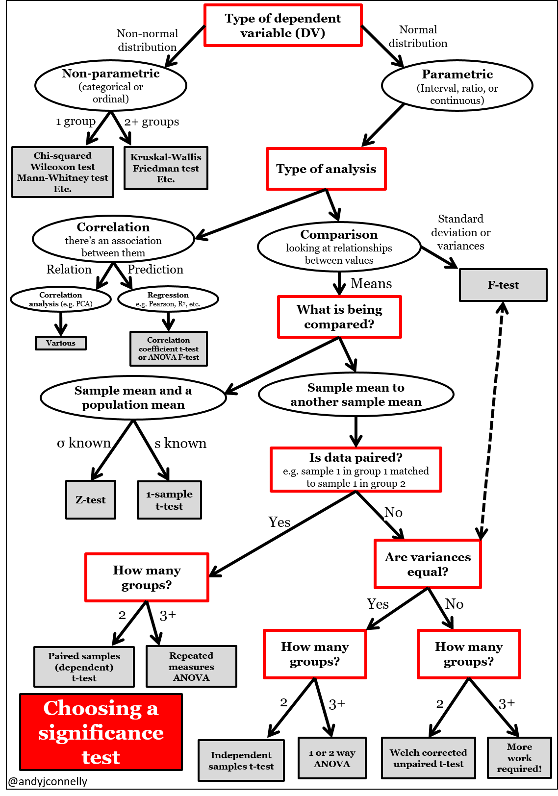
• There are different types of t-test, so we should be aware of which t-test to choose.

The diagram above briefly shows which significance test to choose from, when you perform statistical hypothesis tests. You can see several types of t-tests, but in this post I will only cover the most fundamental t-tests that are used for comparing two sampes: paired(dependent) t-test, unpaired(independent) t-test

Unpaired t-test

    Unpaired t-test assumes that two sample groups are independent and from an approximately normal distribution. The formula differs depending on the equivalence or variance.

Equal variance

  parameters:

• \(\bar{x_1}, \bar{x_2}\) is mean value of group 1 and group 2

• \(n_1, n_2\) are numbers of samples of group 1 and group 2

• t-test statistics value: \(t = \frac{\bar{x_{1}}+\bar{x_{2}}}{\sqrt {s^2\biggl(\frac{1}{n_{1}}+\frac{1}{n_{2}}\biggr)}}\)
  

• pooled sample variance: \(s^2 = {\sum_{i=1}^{n_1} (x_i - \bar{x_1})^2 + \sum_{j=1}^{n_2} (x_j - \bar{x_2})^2\over n_1 + n_2 - 2}\)

• degree of freedom: \(df = n-1\)

R Code

t.test(x, y, alternative = "two.sided", var.equal = TRUE)

# or

t.test(dataset$y1, dataset$y2, data = my_data, var.equal = TRUE)

Non-equal variance

  parameters:

• t-test statistics value: \(d = \frac{\bar{x_1}+\bar{x_2}}{\sqrt{\frac{s_1^2}{n_1}+\frac{s_2^2}{n_2}}}\)
  

• group 1 sample variance: \(s_1 = \frac{\sum_{i=1}^{n_1} (x_i - \bar{x_1})^2}{n_1 -1}\)

• group 2 sample variance: \(s_2 = \frac{\sum_{j=1}^{n_2} (x_j - \bar{x_2})^2}{n_2 -1}\)

• degree of freedom: \(df = {\biggl[\frac{s_1^2}{n_1} + \frac{s_2^2}{n_2}\biggr]\over {\bigl(\frac{s_1^2}{n_1}\bigr)^2\over n_1 - 1} + {\bigl(\frac{s_2^2}{n_2}\bigr)^2\over n_2 - 1} }\)

R Code

t.test(x, y, alternative = "two.sided", var.equal = FALSE)

# or

t.test(dataset$y1, dataset$y2, data = my_data, var.equal = FALSE)

Paired t-test

    Unlike, unpaired t-test, paired t-test is used to compare sample menas of two related(dependent) groups (ex. pair of values; before & after)

parameters:

• t-test statistics value: \(t = \frac{m}{\frac{s}{\sqrt n}}\)
  • \(m\) is the mean difference between two groups
  • \(n\) is the sample size of \(d\)
  • \(s\) is the standard devidation of \(d\)
• \(df\)(degree of freedom) is \(n-1\)

R Code

t.test (Y ~ X, dataset, paired=TRUE)

# or 

t.test(dataset$y1, dataset$y2, paired=TRUE)