Machine Learning Basic

Machine Learning

Machine Learning is a field of computer science that gives computers the ability to learn about being explicitly programmed.” -Arthur Samuel-

Well-posed Learning Problem: A computer program is said to learn from experience E, with respect to some task T and some performance measure P, if its performance on T as measured by P, improves with experience E -Tom Mitchell -

• Machine Learning is providing systems the ability to automatically learn and improve from experience (data)
• It is a field of artificial intelligence research method
• The concept is relevant to how humans learn and perceive matters
• Most of its methods can be summarized or simplified into finding patterns from sample data and classifying them
• It can be used for prediction, or finding meaningful insights ( just like humans learn from their past experience)

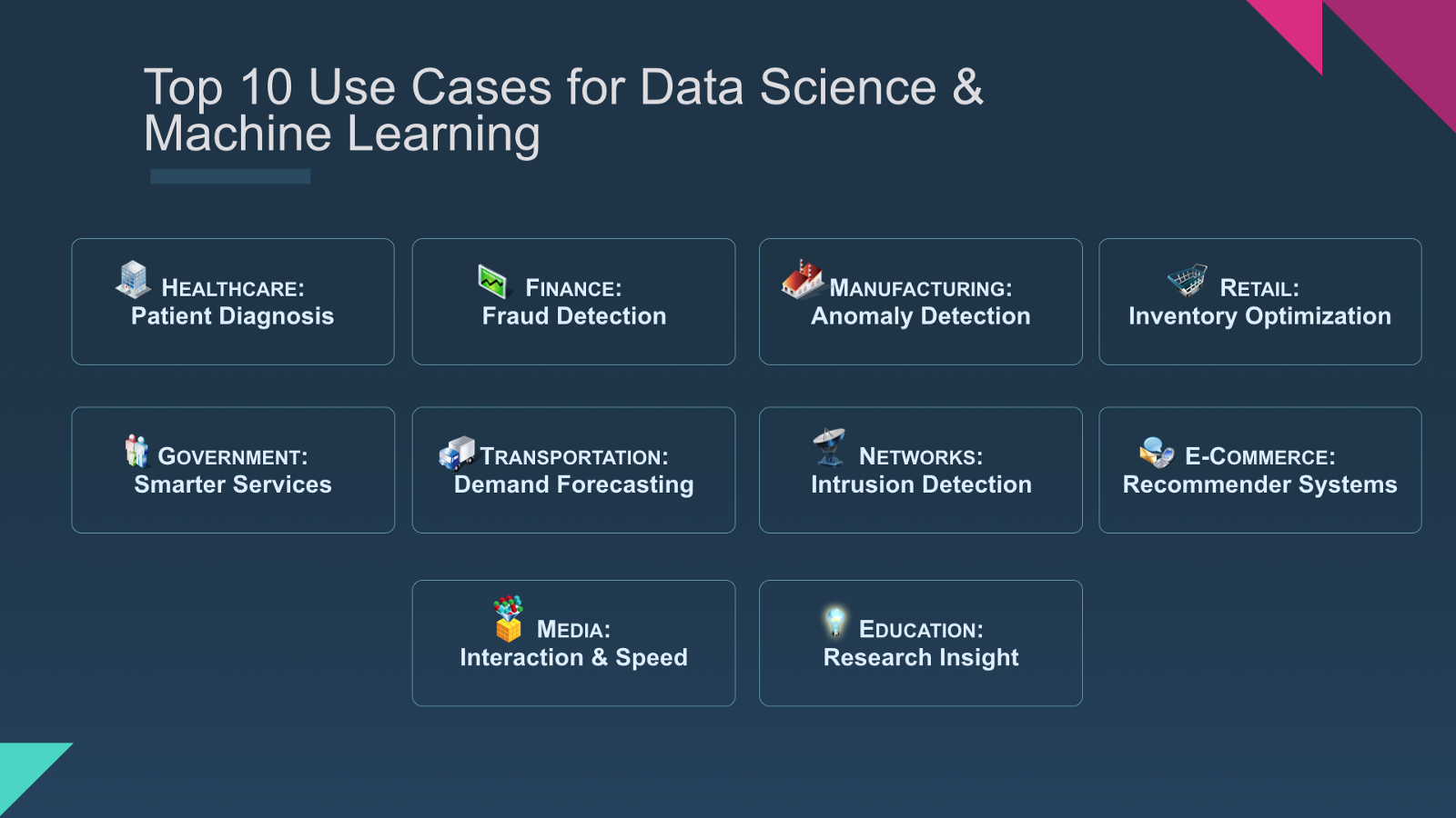
Application of Machine Learning

Types of Machine Learning

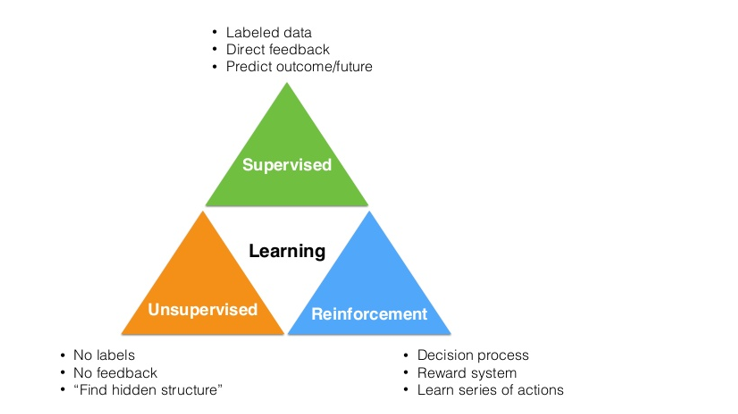
The three most distinctive types of machine learning are:

• Supervised Learning (Classification)
• Unsupervised Learning (Clustering)
• Reinforcement Learning    

Supervised Learning

Supervised Learning trains model or computer with sample data that has labels (or answers). After the labeled data is trained, another data is used to predict label values (or correct answers).

For example, supervised learning provides data like above. The data includes hand-written numbers. With supervised learning, you can train computer with this dataset, and test them with your handwritten numbers whether the computer can recognize them correctly(predicting labels).

Algorithms used in Supervised Learning

• Support Vector Machine (SVM)
• Hidden Markov Model
• Regression
• Neural Network
• Naive Bayes Classification
• KNN Classification …..

Unsupervised Learning

Unsupervised Learning on the other hand, is learning method that does not have any labels or answers. It is used to search for the existence of pattern or clusters in the data.

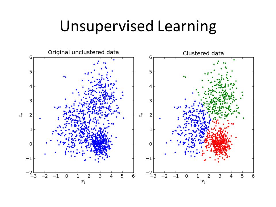
Just as the example above, unsupervised learning is used to find patterns, groups, clusters from data with no specific labels or information

Algorithms used in Unsupervised Learning

• K-means Clustering
• Hierarchical Clustering
• Mean-Shift Clustering ….

Difference between Supervised Learning and Unsupervised Learning

The key difference is in the “labeling”. For supervised learning, we provide dataset with labels or answers. On the other hand, the unsupervised learning does not have labels. The computer automatically split or generate groups (clusters) in accordance to the data features.

<img src=”/assets/images/sup_vs_unsup.jpg>

Reinforcement Learning

Reinforcement Learning is quite different from supervised and unsupervised learning. It includes a unique term “reward”. When the subject (agent) analyses(observation) data and make decisions (actions), it gets reward. Then, the subject will make optimal decision that can maximize its reward.

Machine Learning with Python (Iris Dataset)

Python has great libraries and modules that support machine learning. Scikit-Learn a.k.a sklearn is the most representative module. Sklearn also provides basic dataset so that you can practice machine learning

# importing sklearn in python
import sklearn

Let’s try to solve an example with machine learning

The Iris Dataset

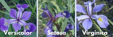    Flower iris has three species: Versicolor, Setosa, Virginica.

The dataset includes 150 different flower data of 4 numeric attributes: sepal length, sepal width, petal length, petal width.

The object is to predict which species group a flower belongs, by building a model with machine learning.

from sklearn import datasets

iris_data = datasets.load_iris()
iris_data

# ['sepal length (cm)','sepal width (cm)', 'petal length (cm)', 'petal width (cm)']

data = iris_data.data

# The Labels:   0 = setosa, 1 = versicolor, 2 = virginica

label = iris_data.target
print(label)

Supervised Learning

In this case, the labels (or answers) would be species name.

KNN-algorithm

knn(k nearest neighbor) algorithm is probably the simplest algorithm in machine learning along with k-means clustering in unsupervised learning.

The algorithm is pretty simple. If k = 3, KNN is deciding a label of new data based on the labels of 3 closest neighbors.

For example, the green circle (data with no label) will be classified as red triangle if k is 3. However, if k = 5, the green circle will be classified as blue square.

Importing KNN library

# KNN model import
from sklearn.neighbors import KNeighborsClassifier

# We are going to split the whole dataset into two groups:
## Train group: training the model 
## Test group: testing the trained model and see its accuracy
### train_test_split allows easy split of the data into train and test groups
from sklearn.model_selection import train_test_split

Splitting Data to train and test set

# Let's set K to 3 ( k = 3)
knnmodel = KNeighborsClassifier(n_neighbors= 3)

# Split the data into train and test
X_train, X_test, y_train, y_test = train_test_split(data,label, test_size=0.3)
# Train data = 70% of whole data
# Test data = 30% of whole data

Training Model

# Train the model
## Your Machine(Model) learns here!!
knnmodel.fit(X_train, y_train)

Prediction and Score

# Let's see how well your machine predicts

## Predicted results from your machine(model)
prediction = knnmodel.predict(X_test)

## The answers
y_test


## Score & Feedback
from sklearn.metrics import accuracy_score

my_score = accuracy_score(y_true= y_test, y_pred= prediction)
print(my_score)

Unsupervised Learning

Let’s try unsupervised learning this time.

Let’s assume that we do not know about the labels or the fact that iris is divided into three species. We will use K-means clustering algorithm to find how the flowers can be grouped.

K-means Clustering

K Means Clustering tries to cluster data based on their similarity. In k means clustering, we have the specify the number of clusters we want the data to be grouped into. The algorithm randomly assigns each observation to a cluster, and finds the centroid of each cluster. Then, the algorithm iterates through two steps:

1. Reassign data points to the cluster whose centroid is closest.
2. Calculate new centroid of each cluster.

These two steps are repeated until the within cluster variation cannot be reduced any further. The within cluster variation is calculated as the sum of the euclidean distance between the data points and their respective cluster centroids.

K-means library

# Import KMeans Clustering module
from sklearn.cluster import KMeans  

Model fitting

# We know that the iris has 3 species
kmeansmodel = KMeans(n_clusters= 3)

# Model fitting
kmeansmodel.fit(data)

# Observing 
# Respective cluster centroids
##### [Cluster0  
####   Cluster1, 
####   Cluster2]
centroids = kmeansmodel.cluster_centers_
print(centroids)

Results

# Let's see how our model clustered the data
print(kmeansmodel.labels_)
print("\n")
print(label)

# REMEMBER! KMeans is not classification. 

Visualizing the clusters

We are going to use PCA(Principal Component Analysis), to fit our data into 2D shape. PCA is a statistical procedure that uses an orthogonal transformation to reduce dimensions.

For example, our iris data has 4 features. We cannot plot them in our graph. (Assuming that 1 variable = 1 axis, 3 variable is the maximum amount that we can plot into our world). So, we are going to reduce our data into 2 dimensional for easy plotting.

We are just performing the comparison to prove that clustering method is reliable!

Using plotly

# plotly is another visualization library just like matplotlib
import plotly.graph_objs as go
from plotly.offline import init_notebook_mode, iplot
init_notebook_mode()

PCA to reduce dimension for plotting

from sklearn.decomposition import PCA
import numpy as np

pca = PCA(n_components= 2)
# Using x as 1st column feature("sepal length") , y as 2nd column feature ("sepal width")
x = pca.fit_transform(data)[:,0]
y = pca.fit_transform(data)[:,1]

# Add PCA x,y values to the dataset
X = x.reshape(150,1)
Y = y.reshape(150,1)

Original Data

cluster0 = go.Scatter( x = np.reshape(X[label==0],50,),
y = np.reshape(Y[label==0],50,),
name = "Cluster0",
mode = "markers",
marker = dict( size = 10, color = "rgba(15,152,152,0.5)",
line = dict(width = 1, color = "rgb(0,0,0)")))

cluster1 = go.Scatter( x = np.reshape(X[label==1],50,),
y = np.reshape(Y[label==1],50,),
name = "Cluster1",
mode = "markers",
marker = dict( size = 10, color = "rgba(180,18,180,0.5)",
line = dict(width = 1, color = "rgb(0,0,0)")))
cluster2 = go.Scatter( x = np.reshape(X[label==2],50,),
y = np.reshape(Y[label==2],50,),
name = "Cluster2",
mode = "markers",
marker = dict( size = 10, color = "rgba(132,132,132,0.8)",
line = dict(width = 1, color = "rgb(0,0,0)")))

real_dat = [cluster0, cluster1, cluster2]

layout_real = go.Layout(
title = "Actual Groups")

real = go.Figure(data=real_dat, layout = layout_real)

Clustered Data

cluster0 = go.Scatter( x = np.reshape(X[kmeansmodel.labels_==0],50,),
y = np.reshape(Y[kmeansmodel.labels_==0],50,),
name = "Cluster0",
mode = "markers",
marker = dict( size = 10, color = "rgba(15,152,152,0.5)",
line = dict(width = 1, color = "rgb(0,0,0)")))

cluster1 = go.Scatter( x = np.reshape(X[kmeansmodel.labels_==1],38,),
y = np.reshape(Y[kmeansmodel.labels_==1],38,),
name = "Cluster1",
mode = "markers",
marker = dict( size = 10, color = "rgba(132,132,132,0.8)",
line = dict(width = 1, color = "rgb(0,0,0)")))
cluster2 = go.Scatter( x = np.reshape(X[kmeansmodel.labels_==2],62,),
y = np.reshape(Y[kmeansmodel.labels_==2],62,),
name = "Cluster2",
mode = "markers",
marker = dict( size = 10, color = "rgba(180,18,180,0.5)",
line = dict(width = 1, color = "rgb(0,0,0)")))

cluster_dat = [cluster0, cluster1, cluster2]

layout_clus = go.Layout(
title = "Grouped by Cluster Model")

cluster_model = go.Figure(data=cluster_dat, layout = layout_clus)

Visualized graph (original data vs clustered data)

iplot(real)
iplot(cluster_model)